The Breadth-first search algorithm is an algorithm used to solve the shortest path problem in a graph without edge weights (i.e. a graph where all nodes are the same “distance” from each other, and they are either connected or not). This means that given a number of nodes and the edges between them, the Breadth-first search algorithm is finds the shortest path from the specified start node to all other nodes. Nodes are sometimes referred to as vertices (plural of vertex) - here, we’ll call them nodes.

Description of the Algorithm

The basic principle behind the Breadth-first search algorithm is to take the current node (the start node in the beginning) and then add all of its neighbors that we haven’t visited yet to a queue. Continue this with the next node in the queue (in a queue that is the “oldest” node). Before we add a node to the queue, we set its distance to the distance of the current node plus 1 (since all edges are weighted equally), with the distance to the start node being 0. This is repeated until there are no more nodes in the queue (all nodes are visited).

In more detail, this leads to the following Steps:

1. Initialize the distance to the starting node as 0. The distances to all other node do not need to be initialized since every node is visited exactly once.
2. Set all nodes to “unvisited”
3. Add the first node to the queue and label it visited.

4. While there are nodes in the queue:

   1. Take a node out of the queue
   2. For all nodes next to it that we haven’t visited yet, add them to the queue, set their distance to the distance to the current node plus 1, and set them as “visited”

In the end, the distances to all nodes will be correct.

Example of the Algorithm

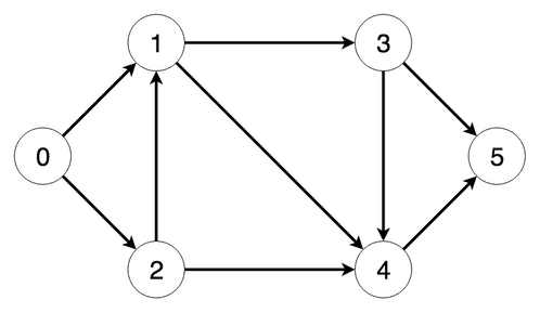
Consider the following graph:

The steps the algorithm performs on this graph if given node 0 as a starting point, in order, are:

1. Visiting node 0

2. Visited nodes: [true, false, false, false, false, false], Distances: [0, 0, 0, 0, 0, 0]

   1. Removing node 0 from the queue…
   2. Visiting node 1, setting its distance to 1 and adding it to the queue
   3. Visiting node 2, setting its distance to 1 and adding it to the queue

3. Visited nodes: [true, true, true, false, false, false], Distances: [0, 1, 1, 0, 0, 0]

   1. Removing node 1 from the queue…
   2. Visiting node 3, setting its distance to 2 and adding it to the queue
   3. Visiting node 4, setting its distance to 2 and adding it to the queue

4. Visited nodes: [true, true, true, true, true, false], Distances: [0, 1, 1, 2, 2, 0]

   1. Removing node 2 from the queue…
   2. No adjacent, unvisited nodes

5. Visited nodes: [true, true, true, true, true, false], Distances: [0, 1, 1, 2, 2, 0]

   1. Removing node 3 from the queue…
   2. Visiting node 5, setting its distance to 3 and adding it to the queue

6. Visited nodes: [true, true, true, true, true, true], Distances: [0, 1, 1, 2, 2, 3]

   1. Removing node 4 from the queue…
   2. No adjacent, unvisited nodes

7. Visited nodes: [true, true, true, true, true, true], Distances: [0, 1, 1, 2, 2, 3]

   1. Removing node 5 from the queue…
8. No more nodes in the queue. Final distances: [0, 1, 1, 2, 2, 3]

Runtime Complexity of the Algorithm

The runtime complexity of Breadth-first search is O(|E| + |V|) (|V| = number of Nodes, |E| = number of Edges) if adjacency-lists are used. If a we simply search all nodes to find connected nodes in each step, and use a matrix to look up whether two nodes are adjacent, the runtime complexity increases to O(|V|^2).

Depending on the graph this might not matter, since the number of edges can be as big as |V|^2 if all nodes are connected with each other.

Space Complexity of the Algorithm

The space complexity of Breadth-first search depends on how it is implemented as well and is equal to the runtime complexity.